The Price of Sparsity

Two true things in the world: learning comes from compression, and models should be sparse. In this post, we will talk about the latter, focusing on the training techniques for sparse models.

0. Motivation

Training large models is costly. Making models sparse (e.g., by setting certain weights to be constantly zero, which is effectively removing them) can accelerate both training and inference, saving a lot computation. We refer to this process as sparse training. Our objective is to train sparse neural networks with matching generalization performance as their dense counterparts, even at a very high sparsity level.

1. Backgrounds

The above is a challenging task due to the fundamental tradeoff between efficiency and performance (cf. the rate distortion tradeoff, [Dai at al., 2018] and [Gao et al., 2019]). That being said, while higher sparsity level implies higher computational efficiency, it is often brings performance degradation.

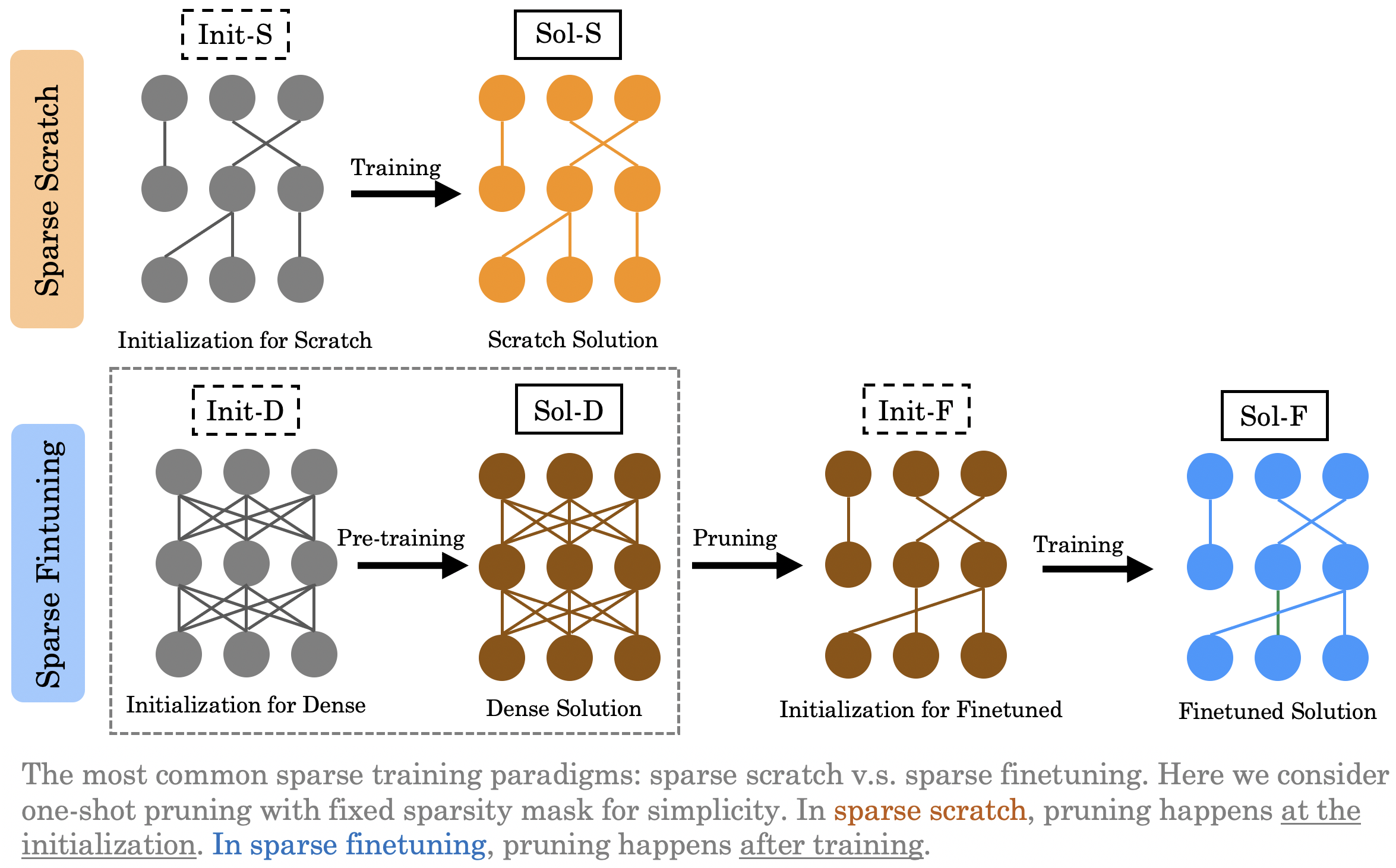
The most efficient approach is to directly train a sparse neural network from scratch (a.k.a., sparse scratch, or pruning at initialization, as depicted by Init-S -> Sol-S above). However, in practice, it often results in relatively low generalization performance. People find that it is often better to first pre-train on a dense network, then to prune the trained solution, and finally to finetune on the resulting weights (a.k.a., sparse finetuning, or pruning after training, as depicted by Init-D -> Sol-D -> Init-F -> Sol-F).

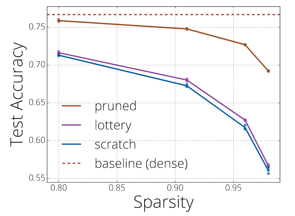
In [Evci et al., 2020], the authors compare sparse scratch and sparse finetuning, and find that even with the same pruning mask (which means the only difference lies in their initializations, Init-S and Init-F), the former still perform worse than the latter. The below figure is extracted from [Evci et al., 2020], where pruned corresponds to our sparse finetuning and scratch corresponds to our sparse scratch, and lottery additionally involves an iterative process. Our verification of this phenomenon will be presented in the next section. The high-level message here is that there is a generalization performance gap between sparse scratch and sparse finetuning.

This is not good. Sparse finetuning is a tortuous path and is still very computationally expensive. Is there a way for us to get rid of the dense pre-training phase while still achieving comparable generalization performance?

Things are not desperate.

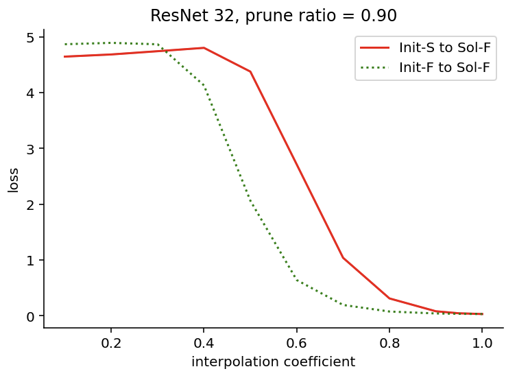
In the above figure, we show that there exist a path, from Init-S to Sol-F, where the loss is almost monotonically decreasing (first discovered in [Evci et al., 2020]; the loss on the y-axis is computed by linearly interpolating between Init-S and Sol-F). This means that it is possible for sparse scratch to have the same results as sparse finetuning.

2. The Quest

Before we can reach the same performance as dense training, let’s first make sparse scratch being on par with sparse finetuning, which would already provide us with remarkable efficiency in practice.

We thus ask the following research questions:

• What is the root cause for the performance gap between sparse scratch and sparse finetuning?
• How can we close the performance gap?

For the first question, the secrets lies in the training dynamics. One of the most fundamental and general way to depict the training dynamics, from my own perspective, is by information measures, which is easy for humans to understand and help design principled training approach. We will go in depth later, but as a teaser here, Fisher information is a local discrepancy measure for the prediction distribution of neural networks, and we found the Fisher information for sparse scratch is much higher than that of sparse finetuning. This simple metric unveils crucial dynamics impacting both generalization and optimization – see our analysis forthcoming.

For the second question, the strategy is direct: to control (or stabilize) Fisher information. How can we do that? Recall that Fisher information is derived from the prediction distribution, thus so simplest and the most direct way is to adjust the training data distribution fed into the network (e.g., by using data subsets with lower Fisher information in the earlier phase of training). This is just like building a data curriculum as discussed in Bengio et al. (2009), which works like a charm in sparse training.

3. A Tale of Two Regimes

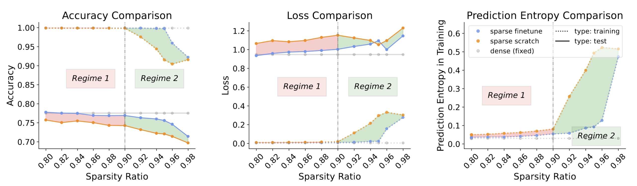
Remember that in Figure 2 (the excerpt from [Evci et al., 2020]) shows that there is generalization gap. We further find that, as the sparsity ratio increases, the generalization gap can be characterized by two regimes:

• the generalization regime
• the optimization regime

To be specific, although there is a persistent generalization gap between sparse scratch and sparse finetuning, the underlying mechanism is different across different sparsity level.

• In regime 1, there exist large generalization discrepancies for sparse-scratch and sparse-finetuning while they maintain almost the same near-optimal training accuracy. We denote this regime as the generalization regime.

• In regime 2, there emerge large discrepancies on training accuracy as well. We denote this regime as the optimization regime.

This observation gives us a convenient way to understand the gap.

• In regime 1 where the sparsity ratio is low, both models are able to fit or memorize all the training data, such that the gap in the test accuracy mainly comes from generalization-related characteristics like the loss curvature.
• In regime 2 where the sparsity ratio is high, sparse scratch cannot fit or memorize certain training data compared to sparse finetuning, thus besides the generalization-related characteristics, the gap also have something to do with the training failure. To close the gap, we need to solve such training failure first.

4. Fisher Information Provides a Unified Explanation

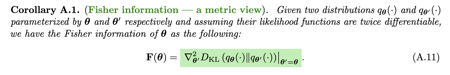
I provide a detaled write-up on understanding Fisher information in the context of deep neural networks at this link. The important message here is that Fisher information should be viewed as a local discrepancy measure of network prediction distribution. Specifically:

If small variation in $\theta$ results in large discrepancy to the network prediction distribution $q_{\theta}(\cdot)$, this $\theta$ can be seen as to withhold high amount of information about the learning process.

I claim that this is the right way to understand Fisher information, instead of the classical parameter estimation view which treats the network parameter $\theta$ as an unknown parameter to be estimated.

We plot the Fisher information curves during training, which have very different behaviors for the two regimes. Here, learning is like crossing an information barrier.

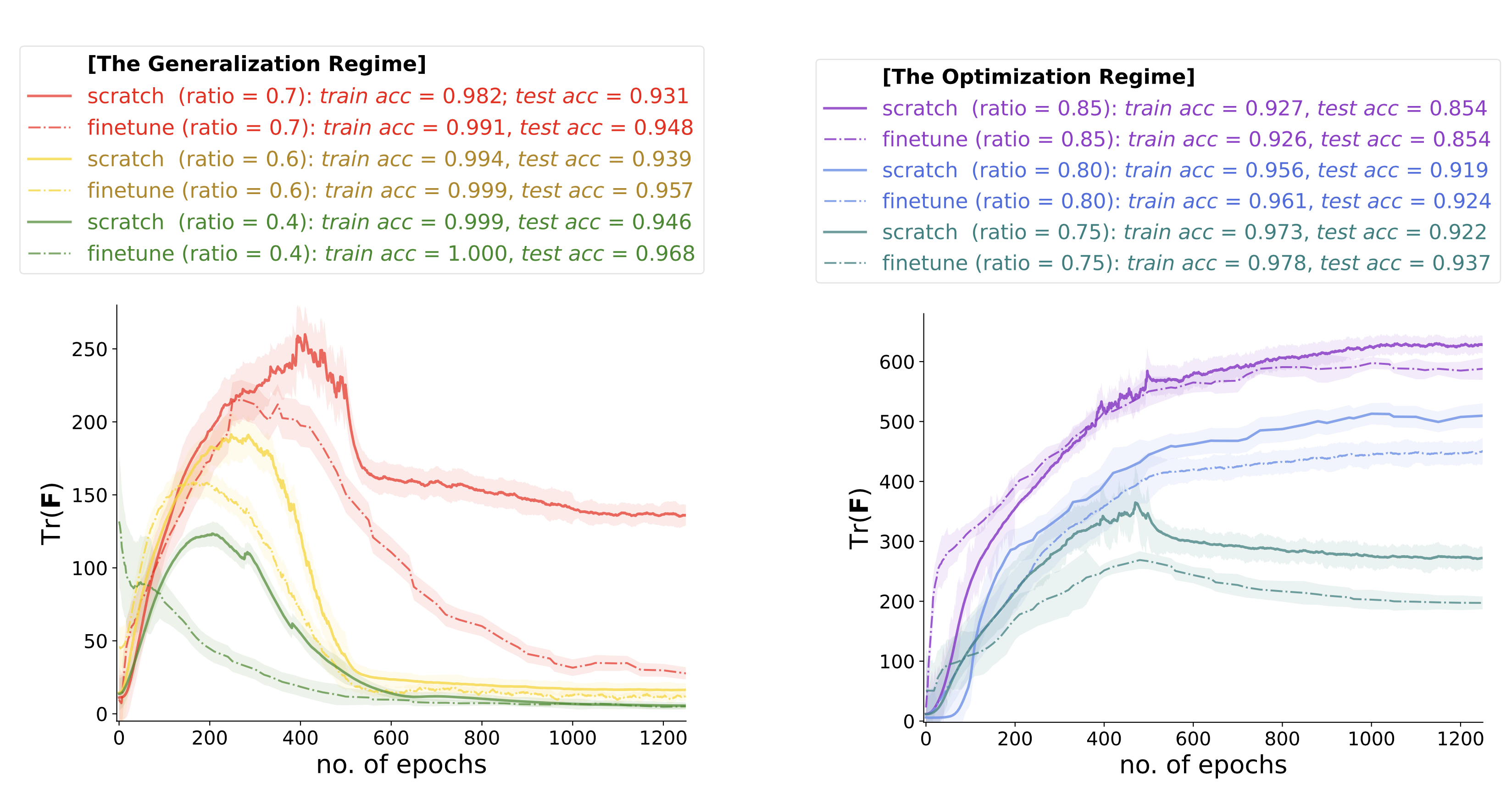
Learning to generalize is like crossing an information barrier. And here are two main messages we learn from the plot:

• The Fisher information curves are different for the two regimes.
• The Fisher information for sparse scratch is always higher than that for sparse finetuning.

This metric view offers a sensible interpretation on common trends of the Fisher information of the network prediction distribution during training. Relatively speaking:

• Low $\textbf{F}_{\theta}$: This implies the gradient update will not change the prediction much. It usually happens at:
  • the initial few steps, where the prediction distribution is close to random, and a small variation to the parameter of the random will have little influence on the distribution.
  • the converging phase, where the training is rather stabilized.
• High $\textbf{F}_{\theta}$: This implies even a small perturbation to the parameter can bring large discrepancy of the network prediction. It is usually happens at the fitting phase, induced by:
  • learning new concepts or difficult examples (cf., [Achille et al., 2019])
  • memorizing noisy examples (cf., [Jastrebski et al., 2021])

This generally explains why the Fisher information is higher for sparse scratch, i.e., some examples are harder to learn or memorize by the network.

• If this happens at the ending epochs, it brings optimization failure, which we observe in regime 2.
• If this happens in the middle of the training, it implies higher training instability and dampens the generalization performance. This mechanism comes from the close relationship of Fisher information and the loss Hessian. See our paper for more detailed discussion.

This indeed provides us with a unified solution for to improve the generalization performance of sparse scratch the both regimes: controling the Fisher information.

5. The Proposed Solutions

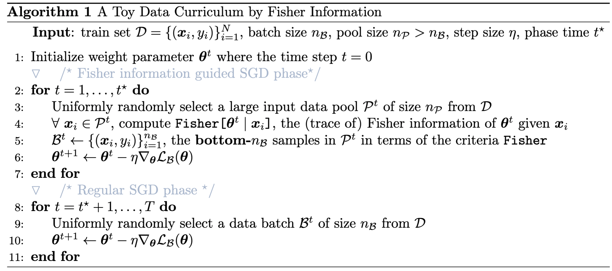
The high level idea here is that we can simply control the Fisher explosion (cf., [Jastrebski et al., 2021]) by directly train with examples with low Fisher information during the critical early stage. Prior works like this include [Paul et al., 2022], which considers to find lottery ticket with less dense pretraining steps by training with only easy examples (filtered by the error L$^{2}$-norm score as in [Paul et al., 2021]).

Notes

1. The title is a tribute to The Price of Salt.
2. Traditional GPUs are optimized for dense computations. For sparse training to be really useful, it is necessary to improve such hardware support as well, e.g., they should be able to handle sparse matrix operations and optimize for the memory access pattern.
3. In this paper, our pruning procedure is confined to one-shot pruning; the next step is to extend to multi-shot pruning (e.g., iterative pruning like in lottery tickets or dynamic pruning). Rewinding is a very beautiful concept. We would also extend the pruning criteria (currently we use magnitude-based approach; we can consider gradient-based approach etc).
4. We plan to extend to work from classification tasks to generation tasks as well (e.g., on both stable diffusion and LLAMA).
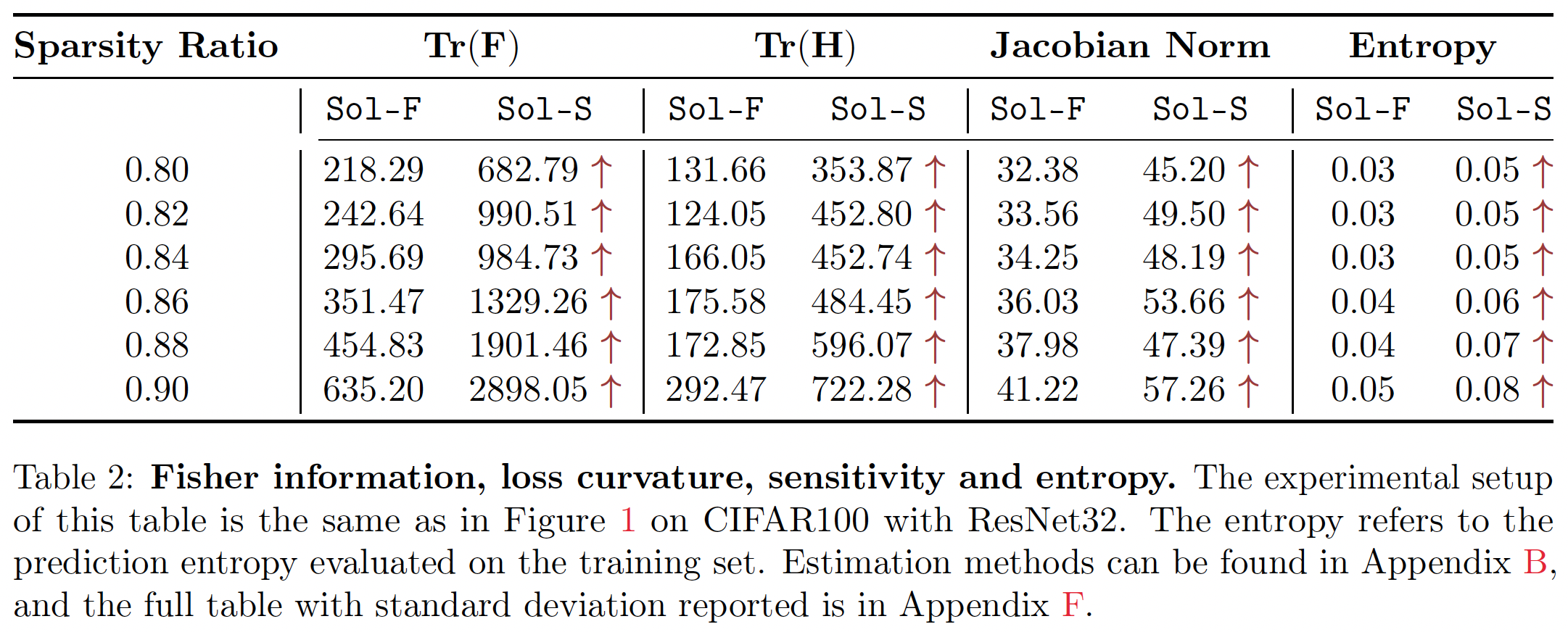
5. Fisher information has close relationship to loss curvature (i.e., Hessian, which is defined to be $\mathbf{H}(\boldsymbol{\theta})=\nabla_{\boldsymbol{\theta}}^2 \mathcal{L}(\boldsymbol{\theta})$) and parameter sensitivity (i.e., Jacobian, which is defined to be $\mathbf{J}(\mathbf{x})=\nabla_{\mathbf{x}^{\mathrm{T}}} f(\mathbf{x} ; \boldsymbol{\theta})$), which were found to be relevant to the generalization performance. Below is our empirical findings.

1. After this paper, we found that sparsity scratch brings quantum enhancement (cf., [Liu et al., 2023]). Firstly, sparsity first allows for a practical interface between classical and quantum devices by efficient uploading through QRAM; secondly, the resulting dissipative nature of the network in the early stage (i.e., more positive eigenvalues) brings exponential decay for the linearization error. To be specific, for a neural network with parameter size $n$ and sparsity $s$, running in $T$ iterations, there is a quantum algorithm runs with the error $\epsilon > 0$ and the complexity,

\begin{equation}\frac{s^3 T^2}{\epsilon^2} \operatorname{poly}\left(\log n, \log \frac{1}{\epsilon}\right).\end{equation}

---

• Previous
  Information Directed Sampling Revisited

---